count - counting cells in 2D photographs
Program count is devoted to counting cells or nuclei appearing as bright, oval-shaped objects in two-dimensional
photographs taken by means of microscope. Optimal performance is obtained for nucleus stainings, where nuclei are approximately round
and well distinguished from the background. One encounters such situation frequently while working with good stainings and taking pictures
using a confocal microscope. A great advantage of the program count is that nuclei (or cells) do not need to be
completely separated - they may form some large clusters of objects, and the program's ability in recognizing separate cells is comparable
to that of a human (under certain conditions, of course). When staining are poor, it is still possible to use the program, just by manipulating its parameters.
But the greatest thing is that such a machine counting treats all pictures in the same way - a perfect elimination of so called
human factor
, which leads to an increase/decrease of number of cells according to someone's expectations.
The program is a command-line tool, but is easy to use and can analyze many pictures in a single run.
It can be used, e.g., for fast comparison of the average number of cells in samples taken for mutant/control, to check whether some
statistical difference is present. All results are saved to a file, so that they can be imported and further analyzed e.g. in Excel*.
*I mention here the name Excel
, knowing something about biologists habits,
but I strongly recommend to use a program dedicated to data analysis.
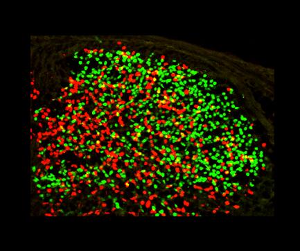
Take a look at the following transversal section of the dorsal spinal cord. It has been stained using antibodies against transcription factors: Tlx3 (green) and Pax2 (red). The picture is taken by confocal microscope.
1. The photo is loaded into computer memory and separated for different channels: red, green and blue. Because we want to count only green cells, red and blue channels are removed. In general, however, the user can choose any single channel, or a combination of them. In case of a combination of two channels, the product of their brightness is taken for further calculations, so that only pixels being bright in both channels contribute. In case if the user chooses all channels, the sum of their brightness is calculated instead of a product. This means that all bright spots will be count, regardless of the channel. The same happens automatically if only a gray-scaled picture is given.
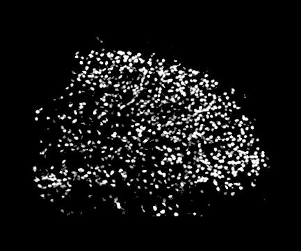
Next, background is removed. This means that all pixels with brightness below some level are rejected. The level is set automatically, or can be given by the user. The picture looks now like this:
2. The program tries to determine the average size of a bright spot
(a nucleus) and all spots which linear size is
below some threshold are rejected (see figure below). This allows one to remove some rubbish present in photographs, or to restrict counting only to cells
above some size. The threshold can be given by the user, or is determined automatically from the average cell size in the picture.

3. Now it comes to the real job. To have the possibility of separating nuclei which overlap a bit, the program blurs
the whole picture in a certain way, so that positions of maxima of brightness indicate now positions of nuclei centers.
This method works well under assumption that nuclei are approximately oval. The following picture explains the idea:

blurredversion (b). One can think of it as a map (c), where points with different brightness have different height (d). Peaks represent approximate centers of nuclei.
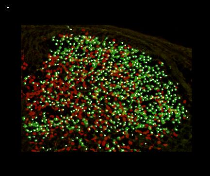
4. Finally, all maxima are counted. If some of them lie very close to each other, the program assumes that they lie within a single nucleus and counts them as a single object. The position of the nucleus center is then calculated as an average of their positions. The minimal distance which indicates that two maxima belong to different nuclei is estimated by the program, or can be explicitly given by the user.
5. The program generates a picture, where positions of all counted objects are marked by white spots. The background is just the photo with properly reduced brightness. In the top-left corner a circle is made indicating what is considered by the program as the average cell size. The picture can be used to check the quality of counting visually.
counting.dat which looks like this: # program COUNT: mode = G # background=60 cut_size=0.5 min.dist.=0.2 # number diameter pixels av. bright. name 633 5.72121 18212 25 pic1.bmp
Even if the picture is good, i.e. the staining has produced bright rounded cells with small background, some cells can be counted incorrectly.
This is because some clusters of objects cannot be separated well using the above method. If you look carefully in the picture, you will
find many cases where a human would probably distinguish cells better than the program. However, the number of such cases,
although it may appear big, is only
a small fraction of all counted cells. Because people usually make several photos to get some averaged
countings and get rid of
some randomness which is always present in living organisms, this is not a real disadvantage since such fluctuations are random and will
be averaged when the number of photos grows.
Moreover, usually one is interested not in absolute number of cells, but rather in its change when compared to a control sample.
Then the above problem becomes even less important. If one assures that all photos are taken at the same conditions, the same staining,
the same preparation of tissue, etc., the program easily finds the difference if it is present. In particular, the counting
of cells made entirely by the human (by eye
counting) leads almost always
to the same result (there is a difference/no difference) as when using the program count. The absolute numbers
can be, however, slightly different in both cases.
When the staining is bad, so that cells or nuclei are perforated
, the results are worse. Not everything is, however, lost. By choosing program
parameters carefully, one can still use it. Below is an example where only red&green = yellow cells were counted.
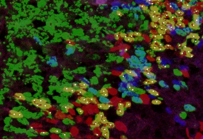
holes, but they are (most of them) counted by the program in a right way. Another example where counting was complicated because of a large overlapping and deformated shape of nuclei:

The first version of this program was written to help my wife, Justyna Cholewa-Waclaw (MDC, Berlin-Buch) in her work. She has prepared many pictures presented here, and helped me to test the program. Encouraged by her interest, and by positive opinions of her colleagues from Department of Developmental Biology and Signal Transduction (group of Prof. C. Birchmeier), I decided to develop the program and to prepare this web page.